Simulating confounders

Let's simulate a confounding relationship now, and see what happens when we test for association. For simplicity we'll use continuous variables and linear regression.

Let's imagine we are interested in the effect of a variable $A$ and an outcome variable $C$. But there is a confounder $B$. What does that do to our association?

We'll simulate a classic confounding relationship like this:

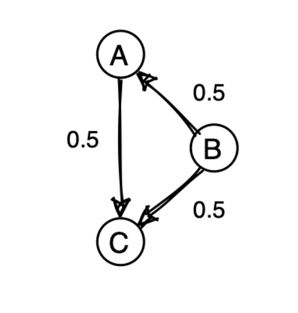
So $B$ affects both the predictor $A$ and the outcome $C$.

Simulating

We'll make this as simple as possible, by making every variable be normally distributed. And all the effect sizes will be 0.5 as indicated in the diagram.

Let's start now, simulating data on $N = 1,000$ samples, say.

N = 1000

First, since $B$ has no edges coming into it, we can simulate it simply by randomly drawing from a normal distribution:

B = rnorm( N, mean = 0, sd = 1 )

Second, since $A$ has only one arrow into it (from $B$), we camn simulate it as $0.5\times B$ plus some noise. To keep things simple, we'll add 'just enough' noise so it has variance $1$ again:

A = 0.5 * B + rnorm( N, mean = 0, sd = sqrt( 0.75 ))

Note

Why the square root of 0.75 here?

Well, $B$ has variance $1$, so $0.5\times B$ has variance $0.25$. If we want to have variance $1$ we have to add on something with variance $0.75$.

Finally, let's simulate $C$. It ought to be made up of a contribution from $A$, a contribution from $B$, and some additional noise:

$$C = 0.5 \times A + 0.5 \times B + \text{noise}$$

How much noise? Again, the contributions from $A$ and $B$ each have variance $0.25$. But they also covary which has to be taken account of. The correct formula works out to be

$$\text{var}(0.5\times A + 0.5 \times B) = 0.25 \times \text{var}(A) + 0.25 \times \text{var}(B) - 0.5 \times \text{cov}(A,B)$$

The covariance is 0.5 so this works out as 0.25:

C = 0.5*A + 0.5*B + rnorm( N, mean = 0, sd = sqrt( 0.25 ))

Let's check this now by computing the covariance between variables.

simulated_data = tibble(
    A = A,
    B = B,
    C = C
)
cov( simulated_data )

You should see something like this:

> cov( simulated_data )
          A         B         C
A 1.0396708 0.5128317 0.7698858
B 0.5128317 1.0058647 0.7557131
C 0.7698858 0.7557131 1.0113318

Naive testing for association

Now let's fit our linear regression model of the outcome variable $C$ on $A$:

fit1 = lm( C ~ A )
coeffs1 = summary(fit1)$coeff
print( coeffs1 )

Question

What estimate do you get for the effect of $A$ on $C$? Does it capture the causal effect? Is it too high? Too low?

Testing for association controlling for confounding

The great thing about regression models is they make it easy to control for confounders - if only yuou have measured them! Here is another linear regression fit that simultaneously fits both $A$ amd $B$ as predictors:

fit2 = lm( C ~ A + B )
coeffs2 = summary(fit2)$coeff
print( coeffs2 )

Question

What estimate do you get for the effect of $A$ on $C$? Does it capture the causal effect? Is it too high? Too low?

Challenge question

Go back and re-simulate the data but having a true effect size of zero between $A$ and $C$. What happens to the estimates now?