Simulating confounders

Let's simulate a confounding relationship now, and see what happens when we test for association. For simplicity we'll use continuous variables and linear regression.

Let's imagine we are interested in the effect of a variable $A$ and an outcome variable $C$. But there is a confounder $B$. What does that do to our association?

We'll simulate a classic confounding relationship like this:

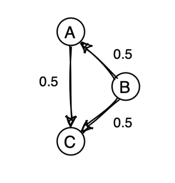
So $B$ is a confounder: it affects both the predictor $A$ and the outcome $C$.

Simulating

We'll make this as simple as possible, by making every variable be normally distributed. And all the effect sizes will be 0.5 as indicated in the diagram.

Let's start now, simulating data on $N = 1,000$ samples, say.

N = 1000

First, since $B$ has no edges coming into it, we can simulate it simply by randomly drawing from a normal distribution:

B = rnorm( N, mean = 0, sd = 1 )

Second, since $A$ has only one arrow into it (from $B$), we can simulate it as $0.5\times B$ plus some noise. To keep things simple, we'll add 'just enough' noise so it has variance $1$ again:

A = 0.5 * B + rnorm( N, mean = 0, sd = sqrt(0.75) )

Aside on variance computations

It turns out that adding something with variance $0.75$ is just the right thing here to make $A$ have variance $1$ again.

The reason for this is the property of the variance that, if $X$ and $Y$ are independent, then

$$\text{var}(X+Y) = \text{var}(X) + \text{var}(Y)$$

In our case since $B$ has variance $1$, $0.5 \times B$ has variance $0.25$. Therefore to make up to variance $1$ we need to add some independent 'noise' with variance $0.75$. That's what the code above does.

If you want to see more detail on how these variance computations are carried out, see the 'extras' page on computing with (co)variances.

Finally, let's simulate $C$. It ought to be made up of a contribution from $A$, a contribution from $B$, and some additional noise:

$$C = 0.5 \times A + 0.5 \times B + \text{noise}$$

How much noise? Again, the contributions from $A$ and $B$ each have variance $0.25$. But they also covary which has to be taken account of. The correct formula turns out to be

C = 0.5*A + 0.5*B + rnorm( N, mean = 0, sd = sqrt( 0.25 ))

Aside on the calculation

Why is this? Again it uses the basic formula for adding variances:

$$\text{var}(X+Y) = \text{var}(X) + \text{var}(Y) + 2 \text{cov}(X,Y)$$

Here $\text{cov}(X,Y)$ is the covariance between $X$ and $Y$ - a measure of their colinearity (after subtracting the mean).

This and other formula are derived on the computing with (co)variance page.

If you apply this in our example adding up a half of each of $A$ and $B$, it works out as:

$$\text{var}\left(\tfrac{1}{2} A + \tfrac{1}{2} B\right) = \tfrac{1}{4} \text{var}(A) + \tfrac{1}{4} \text{var}(B) + \tfrac{1}{2} \times \text{cov}(A,B)$$

Since $A$ and $B$ both have variance $1$, and since the covariance of $A$ and $B$ is 0.5 because of how we computed $A$, this works out as 0.75. So to make $C$ have variance $1$ again we need to add independent noise with variance 0.25, which is what the line above does.

Let's check this all worked now by computing the covariance between variables.

simulated_data = tibble(
    A = A,
    B = B,
    C = C
)
cov( simulated_data )

You should see something like this:

> cov( simulated_data )
          A         B         C
A 1.0396708 0.5128317 0.7698858
B 0.5128317 1.0058647 0.7557131
C 0.7698858 0.7557131 1.0113318

Does this look right?

Testing for association

Testing without controlling for the confounder

Now let's fit our linear regression model of the outcome variable $C$ on $A$:

fit1 = lm( C ~ A )
coeffs1 = summary(fit1)$coeff
print( coeffs1 )

Question

What estimate do you get for the effect of $A$ on $C$? Does it capture the causal effect? Is it too high? Too low?

How confident is the regression in this estimate (e.g. how small is the standard error, or how low is the P-value?)

Testing after controlling for the confounder

The great thing about regression models (as opposed to to things like, say, T tests or 2x2 tables) is that they make it easy to control for confounders. Let's fit another linear regression fit that simultaneously fits both $A$ and $B$ as predictors:

fit2 = lm( C ~ A + B )
coeffs2 = summary(fit2)$coeff
print( coeffs2 )

Question

What estimate do you get for the effect of $A$ on $C$? Does it capture the causal effect? Is it too high? Too low?

Is the estimate within a 95% interval of the true causal effect (i.e. of $0.5$?)

Congratulations! By this point you should understand the basic concepts behind confounding and how they link to regression estimates. To check your understanding, try this challenge question:

Challenge question

Suppose we go back and re-simulate the data but having a true (causal) effect size of zero between $A$ and $C$.

Draw the causal diagram and explain what you think will happen to the estimates now.

Now go back and re-simulate this scenario to confirm your expectations.

Your solution

Try this for yourself! If unsure, you can look at the hints.

Hint 1

Draw the causal diagram between $A$, $B$, and $C$. What is the causal relationship between $A$ and $C$? What paths through the graph will be picked up by the association test between $A$ and $C$?

Hint 2

To simulate, you need to re-simulate $C$ according to the formula:

$$C=\frac{1}{2}B + noise$$

...and keep things so that $C$ has variance $1$.

What variance of noise do you need to add to $C$ to do this?

Hint 3

You need to re-simulate $C$, according to the formula:

$$C=\frac{1}{2}B + noise$$

so that $C$ has variance $1$.

What variance of noise do you need to add to $C$ to do this?

Well according to the properties of the variance:

$$\text{var}(C) = 0.25 \times \text{var}(B) + \text{var}(noise)$$

...and of course $\text{var}(B) = 1$ because that's how we simulated it.

So what variance does the noise need to have?

Solution

The causal diagram now looks something like this:

$$A \leftarrow B \rightarrow C$$

There is no causal relationship between $A$ and $C$, but $B$ is a confounder - a variable that affects both $A$ and $C$. You can expect that - if not controlled for - association between $A$ and $C$ will pick up the path through $B$.

To confirm this, you need to re-simulate $C$, according to the formula:

$$C=\frac{1}{2}B + noise$$

so that $C$ has variance $1$. What variance of noise do you need to add to $C$ to do this?

Well according to the properties of the variance:

$$\text{var}(C) = 0.25 \times \text{var}(B) + \text{var}(noise)$$

...and of course $\text{var}(B) = 1$ because that's how we simulated it.

So this means the noise should have variance 0.75 - the R code is:

C = 0.5 * B + rnorm( N, sd = sqrt(0.75) )

(This was of course just the same calculation we did for $A$ above!)