Analysing sequence data in R

The command-line is great, but if you want to do real analysis you need a real programming language.

Let's now load the sequence into R's memory and take a closer look at it. To help with this, we have created a small R package called mscgm that can be used to load the file into R. To install it, run the following in your R session:

install.packages(
    "https://www.chg.ox.ac.uk/bioinformatics/training/msc_gm/2024/code/mscgm.tgz",
    type = "source",
    repos = NULL
)

You should see some messages about downloading and installing the package. At the end it should say something like:

* DONE (mscgm)

Congratulations! You have installed the mscgm package. Let's use it to load the FASTA data now:

fasta = mscgm::load_fasta_to_list( "Homo_sapiens.GRCh38.dna.chromosome.19.fa" )

It will bring a bunch of messages, and hopefully say 'success!'.

The function has returned an R list object. Let's just get the sequence for chromosome 19 out:

sequence = fasta[['19']]

Let's look at the sequence now:

print( sequence )

[1] "N" "N" "N" "N" "N" "N" "N" "N" "N" "N"
(etc)

N's again! Let's find those same bits of sequence we looked at before. The sequence lines in the original file happened to be 60 characters long, so the bases on lines 2001-2023 would be bases 120001 onwards:

print( sequence[120060:120160] )

Counting nucleotides

How many bases are in the sequence? Use length():

length( sequence )

To see how many of each type of nucleotide is in the sequence, we can use the R function table():

nucleotides = table( sequence )
print( nucleotides )

This might take a minute to compute - you should get something like this:

       A        C        G        N        T 
15142293 13954580 14061132   176858 15282753

Finally let's create a barplot to visualise this:

barplot( nucleotides )
grid()

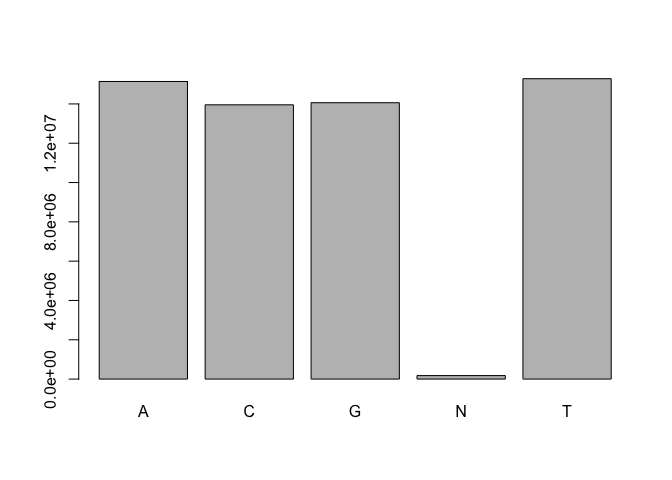
OK cool! So, there are about 200,000 N nucleotides, which form the minority of all the other bases.

Improving the plot

Hmm, it's actually a bit hard to read the values off that plot, because the counts are so different to each other. Let's try using ggplot to plot on a log scale instead. First, put the data into a data frame:

library( tidyverse )
nucleotide_counts = tibble(
    base = names( nucleotides ),
    count = nucleotides
)

Now let's plot it:

p = (
    ggplot( data = nucleotide_counts )
    + geom_col( aes( x = base, y = count ))
)
print( p )

To tidy it up a bit, try theme_minimal():

print( p + theme_minimal() )

Finally let's add the log scale:

print(
    p
    + theme_minimal()
    + scale_y_log10()
)

Do you like this version better? The y axis is now on log scale, i.e. each increment is ten or a hundred times higher than the one below. There are over 10 million of each base, but just over 100,000 N's. (As we saw above the number is actually 176,842 - this log scale still doesn't show the number very accurately.)

Counting Ns

It would be interesting to know the telomere lengths of course - or, in this file, the length of the segment of Ns at either end. To find that out, let's use the which() function to find out the positions of the non-N bases:

nonmissing_bases = which( sequence != 'N' )

And find the first and last of them. (We'll put these in a data frame because why not? It is such a useful data structure):

tibble(
    telomere = c( "start", "end" ),
    length = c(
        min( nonmissing_bases ) - 1,
        length( sequence ) - max( nonmissing_bases )
    )
)

It looks like the sequence of Ns at the start is exactly 60kb long - the one at the end of sequence is much shorter.

Note

The actual telomeres are composed of TTAGGG repeats and the number of ambiguous 'N' bases at chromosome ends is somewhat artificial, but it helps with bioinformatics applications, such as annotation and alignment.

To check we got this right, let's print sequence fragment 10 bases upstream and downstream of the last N to make sure our calculation is correct:

print( sequence[ 59991 : 60010 ] )

[1] "N" "N" "N" "N" "N" "N" "N" "N" "N" "N" "G" "A" "T" "C" "A" "C" "A" "G" "A" "G"

Bingo! Base 60000 is the last N character.

Computing the GC percentage

Let's now take a look at the main DNA bases, and check if AT and GC are in roughtly 50:50 proportion.

To do this, let's take our table object and first convert it to a data frame another way for easier manipulation. We'll do this now and reformat in a useful way:

counts = tibble(
    chromosome = '19',
    A = nucleotides['A'],
    C = nucleotides['C'],
    G = nucleotides['G'],
    T = nucleotides['T'],
    N = nucleotides['N']
)

Now let's compute GC content:

counts$propn_GC = (counts$G + counts$C) / (counts$A + counts$T + counts$G + counts$C)
counts$propn_AT = 1 - counts$propn_GC
print( counts )

You should get something like this:

# A tibble: 1 × 8
  chromosome        A        C        G        T      N propn_GC propn_AT
  <chr>         <int>    <int>    <int>    <int>  <int>    <dbl>    <dbl>
1 19         15142293 13954580 14061132 15282753 176842    0.479    0.521

Indeed, the ratio of G/C bases to A/T bases on this chromosome is approximately 50:50.

Question

Why are we counting G's and C's together, and A's and T's together?

Let's add some code to present our data in a nicer way and make a barlot to show the relative percentages.

sprintf('AT: %.1f%%', counts$propn_AT * 100 )
sprintf('GC: %.1f%%', counts$propn_GC * 100 )

That's much better! And let's plot it:

barplot(c( counts$propn_GC, counts$propn_AT ), names.arg = c('GC %', 'AT %'))

Note

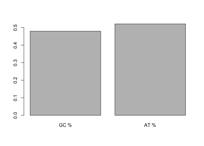
The percentage of GC pairs is referred to as 'GC content'. It varies greatly between organisms and between parts of the genome. It's also a useful QC diagnostic for sequencing runs.

Gene regions tend to have higher GC content; in fact many gene promoters are in CpG islands, which are sequences of CG dinucleotides.

Challenge question

How many CG or GC dinucleotides are there on chromosome 19?